P-values are often mentioned in the scientific literature, but what exactly are they? Short for probability-value, they represent tail-area probabilities of particular distributions and are primarily used in hypothesis testing (for frequentists) and in model checking (for bayesians). In this short post I’ll try to elucidate the two main philosophies on using p-values along with some common pitfalls — the dreaded p-hacking, for instance, along with some pointers on corrections for repeated testing.

(Admittedly, I also have an ulterior motive for this blog post — the simulations I’ll be performing will be done in a Jupyter notebook, and this post will serve as my testbed for Jupyter notebook integration with the Jekyll blogging framework!)

Frequentist perspective on the p-value

A p-value is the tail probability representing the probability of observing replicates that are more “extreme” than the data (with respect to a test statistic) assuming that the null hypothesis were true:

\(\rho = \mathbb{P}(T(D^{rep} > T(D) | \theta),\) where \(D\) is the original dataset, \(D^{rep}\) is a replicate dataset generated according to the distribution \(p(D|\theta)\), \(\theta\) is the true underlying model parameter, and \(T\) is a test statistic of the data.

The point is that if the null hypothesis — represented by the proposed model \(p(D,\theta)\) — were false, then it would be difficult to find data more extreme than what we already observed; that is, that our data is highly “atypical” of what we expect to see from our null model. The p-value \(\rho\) formalizes and quantifies this approach.

In the below, the “null hypothesis” and the “null model” will be treated somewhat interchangeably for two reasons: first, it provides a common vocabulary that bridges the classical frequentist approach and the bayesian approach; second, the null hypothesis statistical testing framework (or NHST) implicitly necessitates a proposal for how the data was generated, i.e. a model. More specifically, however, the null hypothesis will refer to a statement about the parameter \(\theta\) itself and the null model will refer to the proposed joint distribution \(p(D,\theta)\).

Perhaps more important than what a p-value is, is what a p-value is not:

it is not the probability that the null hypothesis is true;
it is not the probability that the alternate hypothesis is true; and
it is not the probability that the dataset comes from a particular model.

The p-value is a proxy to the concordance of the data with the null hypothesis.

So how do frequentists use p-values to critique their null hypothesis? A typical workflow looks something like this:

First choose and fix a null model \(p(D,\theta)\) for data generation with the model parameters \(\theta\) unspecified. The choice of model is important due to the implications it has on the resulting distribution of the test statistic under the null model.
Next, choose a specified significance level \(\alpha\), typically a small value like 0.10, 0.05, or 0.01. The significance level has no intrinsic theoretical significance, but it has an important role to play in as a cut-off between significance and insignificance.
Make a choice of a null hypothesis \(H(\theta)\), for instance \(\theta = 0\) or \(\theta > 0\). The negation of the null hypothesis is called the alternate hypothesis.
The choice of null hypothesis and null model informs the choice of a test statistic \(T(D)\); you want a test statistic which is “sensitive” to the underlying true parameter \(\theta\).
Derive the cumulative distribution function \(F_T(D)\) of the test statistic under the assumption that the null hypothesis is true.
Compute the tail probability (AKA p-value) \(\rho = 1-F_T(D)\) and compare it with the desired significance \(\alpha\).
If \(\rho < \alpha\), reject the null hypothesis with significance \(\alpha\); otherwise, say that we fail to reject the null hypothesis.

It’s important to not overinterpret the meaning of this test. The NHST framework is a way of presenting statistical evidence but does not in itself prove that the either null or alternate hypothesis is true. It is very possible that the dataset is merely atypical, and other factors such as adequate sample size are crucial to our ability to make a strong claim one way or the other.

[IPython] Simulating the null hypothesis significance testing framework.

We wish to demonstrate the following:

\(p\)-values are uniformly distributed when the null hypothesis is true (and all of the test assumptions hold); and
that the distribution is no longer uniform when the above fails.

We’ll base our example around a double-sided t-test; in particular, our population will be infinite and represented by a Normal distribution with variance \(\sigma^2 = 10\) and mean \(\mu = 0\), both of which we pretend not to know. Our hypotheses are as follow:

\(H_\emptyset\): the population mean is zero (\(\mu = 0\)).
\(H_A\): the population mean is nonzero (\(\mu \neq 0\)). The resulting test statistic is then given by \(t = \frac{\hat{\mu} - 0}{\hat{\sigma} / \sqrt(n)}\) where:
\(\hat{\mu}\) is our sample-based estimate of the population mean;
\(\hat{\sigma}\) is our sample-based estimate of the population standard deviation;
\(n\) is the number of elements in our sample;
and \(t\) is the \(t\)-statistic, whose distribution (in our case) is the Student-t distribution with \((n-1)\) degrees of freedom

# Define global constants specifying the population parameters:
# ...In "real life", these parameters would be unknown and answering questions about them
# is the point of statistical hypothesis testing.
POP_MEAN = 0.
POP_VARIANCE = 10.

# Function to generate a random sample from the population:
def get_sample(size):
    return np.random.normal(loc=POP_MEAN, scale=np.sqrt(POP_VARIANCE), size=size)

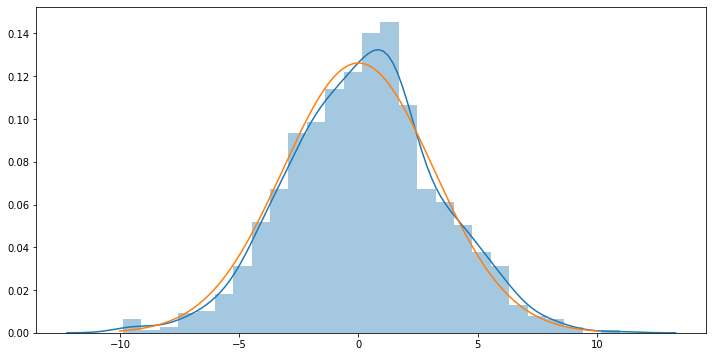
# Verify that we have a sample from a normal distribution (run this cell multiple times until convinced):
plt.figure(figsize=(12,6))
sns.distplot(get_sample(size=1000))
_xs = np.linspace(-10.,10.,num=1000)
plt.plot(_xs, stats.distributions.norm.pdf(_xs, loc=POP_MEAN, scale=np.sqrt(POP_VARIANCE)))

png

# Function to compute the t-statistic of a sample:
def t_statistic(sample):
    return (np.mean(sample) / (np.std(sample) / np.sqrt(sample.shape[0])))

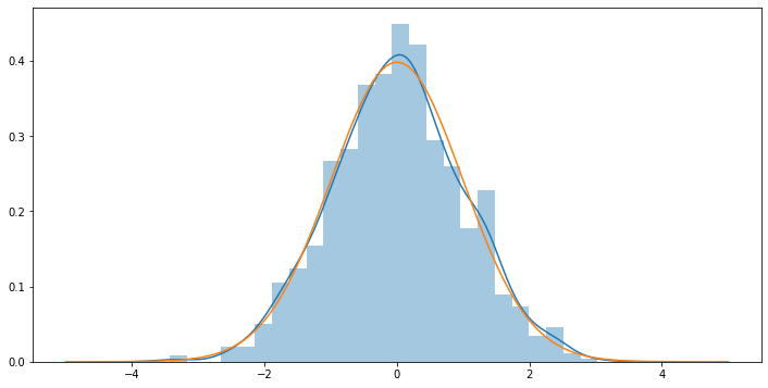
# Verify that we have a t-distribution with df = 99 (run this cell multiple times until convinced):
_tstats99 = [ ]
for k in range(1000):
    _tstats99.append( t_statistic(get_sample(100)) )
plt.figure(figsize=(12,6))
sns.distplot(_tstats99)
_xs = np.linspace(-5., 5., num=1000)
plt.plot(_xs, stats.distributions.t.pdf(_xs, df=99))

png

# Function to generate a p-value from the t-statistic for a given sample:
def pvalue(sample):
    # compute the t-statistic
    t = t_statistic(sample)
    # compute the integral from t to INFTY or from t to -INFTY:
    df = sample.shape[0]-1
    if t > 0:
        pval = stats.t.sf(t, df) # sf = (1 - cdf)
    else:
        pval = stats.t.cdf(t, df)
    return pval

pvalue(get_sample(100))

0.273423292378857

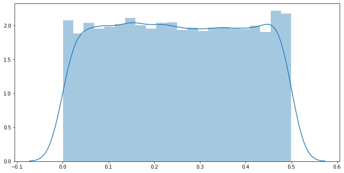
With our hypothesis-testing functions in hand, let’s first plot the distribution of p-values with respect to randomly-generated samples under the assumption that the null hypothesis is true. We can visually confirm that the p-value distribution is in fact uniformly distributed.

# plot the distribution of p-values with respect to randomly-generated samples:
# (We can confirm that p-values are in fact uniformly distributed if the null hyp is true.)
plt.figure(figsize=(12,6))
_pvals = [ ]
for _ in range(10000):
    _pvals.append( pvalue(get_sample(100)) )
sns.distplot(_pvals)

png

# Now let's show how the p-value distribution evolves as we slowly move away from the null hypothesis,
# by varying the mean of our sample away from the population mean:
_alt_hyp_pvals = {'+0.25': [], '+0.5': [], '+0.75': [], '+1.0': [], '+1.25': []}
colors = [ 'r', 'g', 'b', 'c', 'y' ]
plt.figure(figsize=(12,6))
for k,key in enumerate(tqdm(['+0.25', '+0.5', '+0.75', '+1.0', '+1.25'])):
    sample_mean = POP_MEAN + (k+1)*0.25
    for _ in range(10000):
        shifted_sample = sample_mean + get_sample(100)
        _alt_hyp_pvals[key].append( pvalue(shifted_sample) )
    sns.distplot(_alt_hyp_pvals[key], color=colors[k], label=key, hist=False, kde=True)
    print("* Kurtosis = {} for pval dist with sample means = {}".format(stats.kurtosis(_alt_hyp_pvals[key]), key))

 20%|██        | 1/5 [00:02<00:08,  2.21s/it]

* Kurtosis = -1.140121424077413 for pval dist with sample means = +0.25

 40%|████      | 2/5 [00:04<00:06,  2.19s/it]

* Kurtosis = 0.8414760520195985 for pval dist with sample means = +0.5

 60%|██████    | 3/5 [00:06<00:04,  2.19s/it]

* Kurtosis = 8.559498520455355 for pval dist with sample means = +0.75

 80%|████████  | 4/5 [00:08<00:02,  2.21s/it]

* Kurtosis = 53.46836525596685 for pval dist with sample means = +1.0

100%|██████████| 5/5 [00:11<00:00,  2.25s/it]

* Kurtosis = 319.3251033335678 for pval dist with sample means = +1.25

png

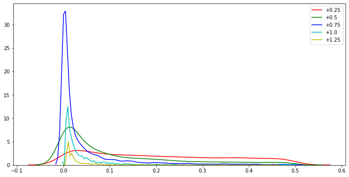
We can notice in the above plot that the p-value distribution gets ‘peakier’ the more we break our assumptions; and this process happens very quickly, with the kurtosis increasing exponentially as we incrementally deviate the sample mean away from the true population mean by 0.25.

(Note that kurtosis is actually a measure of tailedness rather than ‘peakedness’, but the uniform distribution is highly platykurtotic, hence the use of the increasing leptokurtoticity of the p-value distributions as an indicator of deviation from uniformity.)

Now, let’s see what happens to our p-value distribution when we break the assumptions on the sampling distribution.

We’ll compare the p-value distribution from a normal distribution to those of a gamma distribution.

_normal_pvals = []
_gamma_pvals = []

plt.figure(figsize=(12,6))
# run experiment 10,000 times for normal:
for _ in range(10000):
    # compute p-value of t-statistic for normal-dist samples:
    _normal_pvals.append( pvalue(get_sample(100)) )
    # compute p-value of t-statistic for gamma samples:
    _gamma_pvals.append( pvalue(stats.gamma.rvs(1., scale=10., size=100)) )
sns.distplot(_normal_pvals, color='r', label='Normal Samples', kde=True, hist=False)
sns.distplot(_gamma_pvals, color='g', label='Gamma Samples', kde=True, hist=False)
plt.legend(loc='best')

png

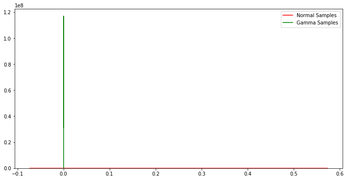
Clearly the p-value distribution is sensitive to the validity of the testing assumptions.

p-values considered harmful?

There are a number of criticisms one may levy against the NHST framework and the present reliance on p-values in the binary decision process for statistical significance. A handful of the more obvious criticisms come to mind:

The NHST framework does not eliminate variance from the statistical model but instead just “hides” it in the seemingly-deterministic decision-making process for determining statistical significance. In practice the designation of significance is not a deterministic decision but rather a sample from a Bernoulli distribution with parameter equal to the significance level. The moral of the story here is that you can’t really eliminate variance from the hypothesis testing process; instead, you’re just hiding it within the Bernoulli.
The common choices of 0.10, 0.05, and 0.01 for a signficance level are essentially arbitrary and a matter of social convention.
Due to the stochasticity of significance testing among replicated datasets, the risk of observing a spurious significant p-value increases as the number of replicates increases. This can happen in subtle ways; for instance, perhaps a dozen researchers replicate a study, but only the one spuriously significant result is published; or perhaps an amateur researcher runs a dozen studies on the same effect and only reports the one spuriously significant study, forgetting to apply corrective measures. We’ll discuss this phenomenon, as well as corrective measures, in the next section.
An indication of statistical significance can itself be scientifically _in_significant. In other words, there are situations where the effect size is minimal — e.g. group A has mean 3.0 and group B has mean 3.1 — but the resulting p-value indicates statistical significance when rejecting equality of group means.
If a p-value smaller than a specified cutoff is all that is needed to have a “gold standard” discovery, then there’s nothing to prevent someone from exhaustively trying dozens and dozens of hypotheses on the same dataset until a spuriously small p-value can be found, i.e. through pure chance alone, the test statistic is located at the tail of the distribution.

That last one is called data-dredging or p-hacking, and is the subject of much criticism and debate.

Abuse of significance testing has led to a so-called “replication crisis” in the sciences, especially in the biological sciences and social sciences. Some notable cases involving the misuse of p-values and the null-hypothesis significance testing framework in general include Carney, Cuddy, Yap (2010) (PDF), which lent evidence to the effectiveness of “power poses” (e.g. “life hacks” like placing your hands on your hips when talking to someone), as well as Bem (2011), which lent evidence to the paranormal notion of precognition — predicting the future. One has to wonder whether, at any point in the study, the authors weighed the likelihood of experimental or procedural errors against the likelihood of the existence of parapsychological phenomena such as precognition.

Multiple comparisons and correction of p-values

P-hacking can be considered in the context of the multiple comparison problem, which is the problem of false discoveries when performing multiple hypothesis tests on the same dataset simultaneously. As an ad hoc example, consider five independent hypothesis tests on the same dataset \(D\), each performed with respect to the same significance \(\alpha = 0.05\). We know that p-values are uniformly distributed with respect to the dataset when the null hypothesis is true — if you generate an infinite number of replicates and compute the p-value of each, the resulting distribution of the p-values is uniform. Hence the probability of at least one false positive is:

\[\mathbb{P}(FP \geq 1) = 1 - \mathbb{P}(FP = 0) = 1 - (0.95)^5 \approx 0.22621 \gg 0.05.\]

In other words, when taken as a whole, the chances of a false positive within the collection of tests somewhere is greater than the threshold \(\alpha\).

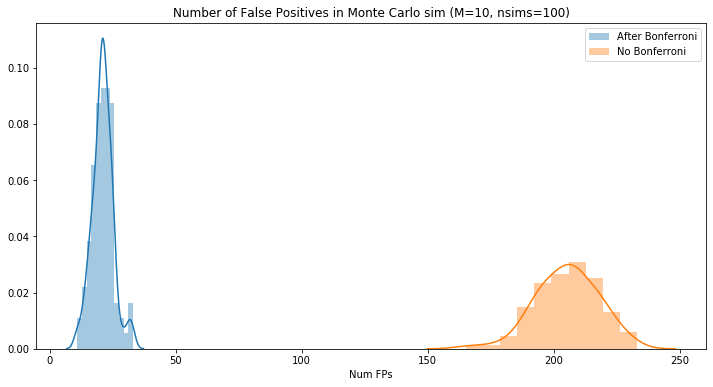
One common way to correct issues arising from multiple hypothesis tests is the Bonferroni correction, which has a very simple implementation. Given p-values \(p_1, p_2, \ldots, p_M\) from \(M\) simultaneous tests at a significance level \(\alpha\), just drop your overall significance level from \(\alpha\) to \(\alpha/M\), i.e. throw away any p-values greater than \(\alpha / M\). One can show that this controls a metric called the familywise error rate, one of many metrics meant to put a figure on the “validity” of your multiple-testing scenario.

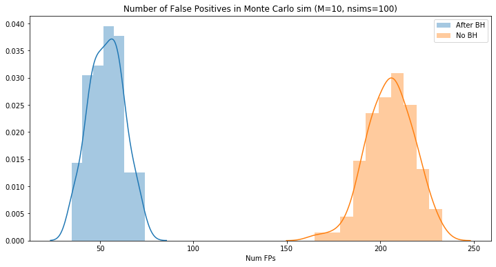
Another correction procedure for multiple testing is the Benjamini-Hochberg procedure, which is designed to control a different metric known as the false discovery rate; the implementation of the Benjamini-Hochberg procedure is a bit more involved but can still be implemented in a few lines of code. The core idea is that the p-values are sorted and everything above a critical p-value is tossed out.

Adjusting for multiple comparisons is a major challenge when one is applying automated, scalable statistical analysis methods to large (terabyte-scale) datasets — for instance, when you have more than tens of thousands of patients in a large healthcare study and each patient has gigabytes of quantitative data across several categories. Multiple testing correction methods like the Bonferroni correction and Benjamini-Hochberg procedure are frequently used to filter away spurious discoveries, but they are also very unforgiving filters that discard many plausible ones. Other methods center on Bayesian approaches and resampling or simulation-based methods. Further work on resolving the problem of spurious correlations will be essential towards the goal of providing automated data analysis backed by well-motivated statistical methodology.

[IPython] Multiple hypothesis testing correction procedures: Bonferroni & Benjamini-Hochberg.

We’ve already demonstrated above that for a given chosen significance level, e.g. \(\alpha = 0.05\), there is a 5% chance that we reject the null hypothesis even if it is true (i.e. a type I error, also known as a false positive or false discovery ). This is obvious given that the p-value distribution is uniformly distributed when the null hypothesis is true and all testing assumptions are valid.

We now demonstrate the flaws in repeating a large number of statistical tests; in particular, we will show that the probability of a false discovery increases with the number of tests. This can be a major flaw when applying large-scale automated statistical testing and may have grave consequences (e.g. in healthcare).

We will also show the results when we apply the Bonferroni and the Benjamini-Hochberg corrections, the two most popular correction procedures that fix the multiple testing problem.

Our demonstration of the pitfalls of multiple testing is based on the following (possibly contrived) anecdote: suppose we had measurements \(y_{i,j}\) for \(i=1,\ldots,10\) representing ten genes with \(j=1,\ldots,J\) datapoints from each gene. The data is normally distributed:

\[y_{i,j} \sim \mathcal{N}(\mu_i,\sigma_i^2),\]

where \(\mu_i\) and \(\sigma_i\) are unknown for each \(i\) — although since this is a contrived example, we have “behind the scenes” knowledge that each \(\mu_i\) is zero and we fix the values of the \(\sigma_i\)’s to be in the range \([1,5]\). Suppose, as before, we want to test whether \(\mu_i = 0\) for each \(i\); our null hypothesis is \(\mu_i = 0\) with significance \(\alpha = 0.1\).

This gives us the following test statistic:

\[t_i = \frac{\sum_j y_{i,j}}{\mbox{s.d.}(y_i) / \sqrt{J}}\]

and the distribution of each \(t_i\) under the null is the student’s t-distribution with \(df = J-1\).

First, let’s write a Monte Carlo simulation scheme to perform ten tests simultaneously and return a vector of ten p-values:

MHT_STDDEVS = [ 1.0, 2.0, 3.0, 4.0, 5.0, 5.0, 4.0, 3.0, 2.0, 1.0 ]
MHT_MEANS = [ 0.0 for _ in range(10) ]

def multiple_tests(means=MHT_MEANS, stdvs=MHT_STDDEVS, sample_size=30):
    """
    Run ten simultaneous tests on a dataset generated by the model above.
    """
    pvals = []
    for i in range(10):
        # generate data:
        yi = stats.norm.rvs(loc=means[i], scale=stdvs[i], size=sample_size)
        # compute test statistic:
        tstat = np.mean(yi) / (np.std(yi) / np.sqrt(sample_size))
        # compute p-value:
        df = sample_size-1
        pv = stats.t.sf(tstat, df) if (tstat > 0.0) else stats.t.cdf(tstat, df)
        pvals.append(pv)
    return np.array(pvals)

# test out our function:
multiple_tests() < 0.1

array([False, False, False,  True, False, False,  True, False, False,
       False])

And now let’s write the function that runs the multiple testing scenario repeatedly and count the number of false positives.

def multiple_testing_monte_carlo(per_test_sig=0.1, nsims=100):
    """
    Run `ntests` tests in parallel at a per-test alpha of `per_test_sig` and
    report the the number of false positives.
    """
    ctr = 0
    for k in range(nsims):
        ctr += np.sum(multiple_tests() < per_test_sig)
    return ctr

print("Number of false positives: {}".format(multiple_testing_monte_carlo(per_test_sig=0.1, nsims=100)))

Number of false positives: 211

The Bonferroni correction procedure focuses on minimizing the family-wise error rate (FWER), which is the probability of making at least one type I error in \(M\) hypothesis tests:

\[\mbox{FWER} := \mathbf{P}(\# \mbox{ (wrongly reject null hyp) } \geq 1).\]

Given an array of p-values from \(M\) tests, the Bonferroni procedure is very easy to implement: just divide your per-test significance level by the number of tests performed; hence if each individual test was performed with a significance level of \(\alpha = 0.05\), to get a FWER of 0.05 on \(M\) tests, throw away any p-value greater than \(\alpha / M = 0.05 / M\).

def bonferroni(pvals, fwer=0.05):
    """
    Args:
    * pvals: NDArray of float type & shape (NTESTS,); the p-values from our tests.
    * fwer: float; family-wise error rate
    
    Returns:
    * correct: NDArray of bool type and shape (NTESTS,); entry k is True if and only
    if pvals[k] passes the correction procedure.
    """
    return (pvals < fwer/pvals.shape[0])

Now let’s see it in action:

def multiple_testing_monte_carlo_bonferroni(per_test_sig=0.1, nsims=100):
    """
    Run `ntests` tests in parallel at a per-test alpha of `per_test_sig`.
    Perform bonferroni correction in the last step of each simulation.
    """
    ctr = 0
    for k in range(nsims):
        ctr += np.sum(multiple_tests() < per_test_sig / 10.0) # divide alpha by M=10 tests
    return ctr

multiple_testing_monte_carlo(per_test_sig=0.1, nsims=100)

multiple_testing_monte_carlo_bonferroni(per_test_sig=0.1, nsims=100)

# plot the distribution of false positives:
mht_bonferroni_fps = []
mht_original_fps = []
for k in trange(100):
    mht_original_fps.append(multiple_testing_monte_carlo(per_test_sig=0.1, nsims=100))
    mht_bonferroni_fps.append(multiple_testing_monte_carlo_bonferroni(per_test_sig=0.1, nsims=100))

100%|██████████| 100/100 [00:54<00:00,  1.88it/s]

plt.figure(figsize=(12,6))
sns.distplot(mht_bonferroni_fps, label="After Bonferroni")
sns.distplot(mht_original_fps, label="No Bonferroni")
plt.title("Number of False Positives in Monte Carlo sim (M=10, nsims=100)")
plt.legend(loc='best')
_ = plt.xlabel("Num FPs")

png

In comparison, the Benjamini-Hochberg procedure focuses on controlling the false discovery rate (FDR):

\[\mbox{FDR} := \mathbf{E}[ \#\mbox{(wrongly reject null hyp) } / \# \mbox{(reject null hyp) } ]\]

…where the ratio inside the expectation is defined to be zero when the denominator is zero.

The Benjamini-Hochberg procedure is less straightforward, but can still be implemented in a few lines of code. The procedure works as follows: for a set of p-values \(\vec{p} = (p_1, \ldots, p_M)\) and their order statistics \(o(\vec{p},1), \ldots, o(\vec{p}, M)\) from smallest p-value to largest p-value, compute the Benjamini-Hochberg critical values

\[BH[o(\vec{p},i)] = \mbox{FDR} * i / M\]

for each index \(i\) and for a chosen FDR representing the largest false discovery rate that you are willing to tolerate. Then, find the largest p-value \(\hat{p}\) that is smaller than its critical value and mark every p-value smaller than or equal to \(\hat{p}\) as significant.

The BH procedure works best when the \(M\) different hypothesis tests are statistically independent. When the tests are not independent, the Benjamini-Yekutieli procedure can be used, which is a slight modification of the Benjamini-Hochberg procedure.

def benjamini_hochberg(pvals, fdr=0.1):
    """    
    Args:
    * pvals: NDArray of float type & shape (NTESTS,); the p-values from our tests.
    * fdr: float; the acceptable false discovery rate.
    
    Returns:
    * correct: NDArray of bool type and shape (NTESTS,); entry k is True if and only
    if pvals[k] passes the correction procedure.
    """
    # compute B-H critical values:
    pvals_crit = np.stack([
        pvals,
        (np.argsort(pvals)+1) * fdr/pvals.shape[0],
    ], axis=1)
    # compute largest p-value that doesn't exceed its critical value:
    if len(pvals_crit[pvals_crit[:,0] < pvals_crit[:,1], 0]) == 0:
        return np.array([])
    else:
        max_crit_pval = np.amax(pvals_crit[pvals_crit[:,0] < pvals_crit[:,1], 0])
    # mark all p-values lower than the largest sub-critical p-value as significant and return:
    return pvals[pvals < max_crit_pval]

# test benjamini-hochberg function:
benjamini_hochberg(multiple_tests(), fdr=0.25)

array([], dtype=float64)

def multiple_testing_monte_carlo_benjamini(per_test_sig=0.1, nsims=100):
    """
    Run `ntests` tests in parallel at a per-test alpha of `per_test_sig`.
    Perform benjamini-hochberg correction in the last step of each simulation.
    """
    ctr = 0
    for k in range(nsims):
        ctr += np.sum(benjamini_hochberg(multiple_tests(), fdr=0.1) < per_test_sig) # apply BH
    return ctr

mht_benjamini_fps = []
for k in trange(100):
    mht_benjamini_fps.append(multiple_testing_monte_carlo_benjamini(per_test_sig=0.1, nsims=100))

100%|██████████| 100/100 [00:29<00:00,  3.64it/s]

plt.figure(figsize=(12,6))
sns.distplot(mht_benjamini_fps, label="After BH")
sns.distplot(mht_original_fps, label="No BH")
plt.title("Number of False Positives in Monte Carlo sim (M=10, nsims=100)")
plt.legend(loc='best')
_ = plt.xlabel("Num FPs")

png

Bayesian perspective on the p-value

Finally, let’s talk about the role of p-values in the Bayesian context. Rather than being used for statistical decision-making as in the frequentist hypothesis testing context usually employed by scientists, p-values in the Bayesian context are used as a form of model critique — i.e. they are employed as a way to guide the development of a credible, robust probabilistic model.

First, let’s provide some context: in Bayesian statistics, the notion of statisitcal hypothesis testing is generalized by hierarchical modelling in the following sense: a null hypothesis in the NHST framework can be considered a testable claim or statement \(T(\theta)\) (e.g. \(T(D \mid \theta) = \tau\), \(T(D \mid \theta) \geq \tau\), etc for proposed test statistic \(T\) and value \(\tau\)) about the parameters \(\theta\) of a simple statistical model \(p(D \mid \theta)\) of the data \(D\).

In the Bayesian context, though, we often build complicated hierarchical models \(p(D \mid \theta)\) with priors on parameters, possibly hyperpriors, et cetera. The notion of hypothesis testing is thus generalized by model critique, and the null hypothesis is replaced by our hierarchical model. Model critique in the Bayesian context involves choices of testable quantities \(T(D, \theta)\) from which we obtain tail probabilities; if the tail probabilities \(\rho_T\) are too far away from their central value of \(0.5\), we can conclude that the model may be a poor fit for the data.

This leads to the posterior predictive distribution :

\[p(D^{rep}|D) := \int_\Theta p(D^{rep}|\theta) \cdot p(\theta|D)\, d\theta,\]

i.e. the generative distribution for new replicate data averaged over parameters \(\theta\) drawn from the posterior distribution \(p(\theta \mid D)\).

The posterior predictive p-value (PPP) is thus defined as the following tail probability:

\[\rho := \mathbb{P}\biggl( T(D^{rep}, \theta) \geq T(D, \theta) \, \biggl| \, D \biggr),\]

where the replicates \(D^{rep}\) are drawn from the posterior predictive distribution and the parameters \(\theta\) are drawn from the posterior distribution.

So how are PPPs used? In pretty much the same was as p-values are used to critique the null hypothesis in the frequentist NHST framework, PPPs are used to critique the model in the Bayesian modelling framework. An example workflow:

Develop a (possibly hierarchical) model of the data \(p(D,\theta)\) whose fit to the data we want to examine.
Compute the posterior predictive distribution and the posterior distribution.
Choose as many test quantities \(T(D,\theta)\) as you want to have to “debug” your model.
Compute the posterior predictive p-value \(\rho_T\) for each test quantity \(T\).

There are some caveats and differences between posterior predictive p-values in the Bayesian context and p-values in the frequentist context. Most notably, the posterior predictive p-value (as a function of \(D\)) does not follow a uniform distribution under the null hypothesis (i.e. if the model is correct), but rather has a distribution with a central tendency around \(0.50\).

Frequentist and bayesian interpretations of p-values