Let’s say you want to model binary outcomes. This is simple if you want a maximum likelihood estimate of a linear set of weights — just perform a logistic regression. But what do we do if we want to perform Bayesian inference?

In this blog post, we’ll look at how we can fit a Bayesian interpretation onto logistic regression via a novel distribution called the Polya-Gamma distribution. The first section will review two popular ways to model dependent binary outcomes: the logistic regression model and the probit regression model. The latter readily admits a Bayesian interpretation thanks to a convenient link function that allows us to sample from the posterior via a (so-called) data augmentation trick. The former, until recently, did not admit a similar trick due to complications with the form of the logistic function. To permit this approach, we introduce the Polya-Gamma distribution of Polson et al in section 3. Finally, we present a data aumentation trick that permits bayesian inference for the logistic regression model using the novel Polya-Gamma distribution, followed by some concluding thoughts and some references.

(N.B.: the proper spelling for the distribution is “Pólya-Gamma” — named after mathematician George Pólya — but I’ll sometimes spell it as “Polya-Gamma” due to the lack of diacritic markers on my keyboard.)

The logistic model and the probit model

Broadly, there are two popular models for binary outcomes: the logistic regression model, traditionally favored by frequentists, and the probit regression model, traditionally favored by bayesians due to the relative ease of sampling from the posterior.

Formally, we have the following context: say we have \(N \gg 1\) datapoints \(D := \{ (x_1,y_1), \ldots (x_N, y_N) \}\) where each \(x_i \in \mathbb{R}^K\) is a vector of regressors and \(y_i \in \{0,1\}\) is a binary response. Set \(X = \{ x_i \}_{i=1}^N\) and \(Y = \{ y_i \}_{i=1}^N\). Assume that each datapoint \((x,y)\) is generated independently from the same identical process and that random \(y\) is dependent upon deterministic \(x\). Let \(w := (w_1, w_2, \ldots, w_K)\) be a vector of parameters, which relate to \(X\) and \(Y\) in a way dependent upon the model (to be discussed further below).

Bayesian models involve the following three ingredients: a prior \(p(w)\) distribution on the vector of parameters; a likelihood function

also called a sampling or data distribution; and a posterior \(p(w|D),\) which is determined by the form of the above two distributions.

The three distributions are linked via Bayes’ theorem:

Note that frequentist statistics focus primarily on obtaining point estimates of properties of the likelihood function, e.g.

The probit model and the logistic regression model are examples of generalized linear models (GLMs), a type of model in which the response variables \(y\) are drawn from a known distribution \(F(y; \theta)\) in which the parameters \(\theta = (\theta_1, \theta_2, \ldots, \theta_m)\) defining the distribution is known, deterministic function \(\theta = g^{-1}(\psi)\) of the linear combination \(\psi := x^\top w\). In other words, we add a “nonlinear layer” on top of the linear combination \(\psi\) to pick a particular distribution

from which we draw \(y\). \(F\) is called distribution of the GLM and \(g\) is called the link function.

For the probit regression model, we use \(g(q) = \Phi^{-1}(\psi)\) the inverse CDF of the standard normal, and \(F = Bern(q)\); this gives us

and a likelihood function

For the logistic regression model, we use \(F = \mbox{Bern}(\sigma(\psi))\) for inverse link function \(\sigma\) the logistic function (hence the name):

Note also that this means we can interpret \(\psi\) as the log-odds of the parameter \(q\) for \(F = \mbox{Bern}(q)\), as we have

For the logistic regression model, we obtain the following likelihood:

Bayesian inference for the probit model via data augmentation

Why do bayesians prefer the probit regression model over the logistics regression model? A major reason is due to the data augmentation strategy developed by Albert & Chib (see references) that allows for efficient sampling from the posterior distribution \(p(w|D)\), which in turn relies on the smoothness of the density of the normal distribution.

Fundamentally, note that the probit regression model in the previous section can be equivalently expressed as a hierarchical latent variable model:

…where we’ve used the Iverson bracket \([u_i > 0]\) to indicate a binary function equal to one if and only if the statement inside the bracket is true.

Why is this equivalent to the probit regression model? The key is to notice that

which gives the equivalence between the latent variable model and the original statement of the probit regression model using the Bernoulli distribution.

Finally, this gives an efficient Gibbs sampler for the posterior \(p(w | X, Y)\) when the prior \(p(w)\) is normally distributed, thanks to the fact that the normal distribution is conjugate to itself: if we place a normal prior \(w \sim \mathcal{N}(\mu_w, \Sigma_w),\)

then the following alternating sampling steps constitute a Gibbs sampler for the posterior:

where

For the full derivation of the above Gibbs sampler, consult Albert & Chib (1993), which was the first to derive the strategy.

The Polya-Gamma distribution

It’s difficult to use the same data augmentation trick to perform posterior inference for the logistic model, which in the latent variable formulation assumes that errors in the latent variable are distributed as a logistic rather than a normal:

where the density of the standard logistic distribution is given as

the logistic distribution is so named because the CDF of the standard logistic distribution is the logistic function \((1+\exp(-x))^{-1}\).

Ease of interpretation may seem like a good reason to use probit regression — and indeed this is frequently a good justification — but it can sometimes be advantageous to use a platykurtotic distribution, or a distribution with heavier tails than the normal. Hence we’d like to have an efficient Gibbs sampler for logistic regression in the same way that we have an efficient Gibbs sampler for probit regression.

For a long time, there was no way to efficiently generate exact samples from the posterior in the logistic regression model; instead, one had to use approximate methods like variational bayes or approximate sampling methods. This led to the preference for the probit regression model over the logistic regression model among bayesian statisticians. Recently, however, a paper by Polson, Scott, & Windle introduced a class of Polya-Gamma distributions — denoted \(PG(b,z)\) for positive integral \(b \in \mathbb{N}\) and continuous \(z \in \mathbb{R}\) — which enable a Gibbs sampler by representing the logistic regression model using a \(PG(b,z)\)-distributed latent variable instead of a logistic-distributed latent variable; this is the subject of the next section of this post.

Formally, the class of Polya-Gamma distributions is equivalent in law to an infinite mixture of Gamma distributions:

where the equality refers to equality of distributions (i.e., in law), and the numerators are random i.i.d. draws from the same Gamma distribution:

Indeed, this offers a naive way to sample from \(PG(b,z)\) — sample several times from a gamma and keep a running weighted sum until the running variance falls below a threshold. However a much more efficient sampler based on rejection sampling is given in the paper, following work by Devroye (2009) based on his groundbreaking book on sampling methods. I won’t delve into the details, but a naive Python-based implementation is contained within the accompanying github repo for this blog post.

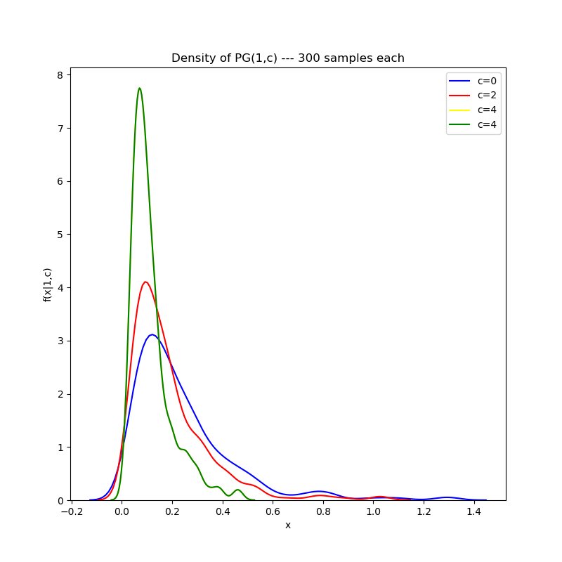
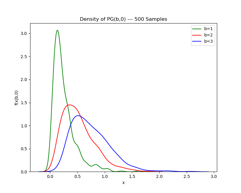
For a glimpse of the \(PG(b,z)\) distribution, I’ve reproduced some of the density plots for varying parameters using my sampler.

First, holding the first parameter constant and varying the second parameter:

Then, varying the first parameter while holding the second parameter fixed:

Note that the aberrations on the tail are due to the kernel density estimation plotting algorithm, which draws a density by fitting a number of Gaussian kernels to empirical data. The tail may be smoothed out by judicious choice of the bandwidth parameter in the KDE plotting algorithm, but I’ve elected to avoid doing this for the purposes of this post.

Bayesian inference for logistic regression using Pólya-Gammas

What’s notable about the Polya-Gamma distribution is that it allows us to develop a Gibbs sampler for the posterior of the above model, via a latent variable trick much like what we did with the probit model: the paper notes that the Polya-Gamma distribution has the following unique property that facilitate the existence of a Gibbs sampler: for any integer \(b > 0\), let \(p(u)\) be the density of a random variable \(u \sim PG(b,0)\). Then for all \(a \in \mathbb{R}\) and \(\psi \in \mathbb{R}\), the following holds:

where \(\kappa := a - (b/2).\) Further, we have that the conditional distribution \(p(u | \psi) = PG(b,\psi)\) when

This is a useful property because the likelihood of observing a single datapoint in the logistic regression model is given by:

combining this likelihood with the above theorem gives the following Gibbs sampling strategy:

where

In python, the above can be implemented in thirteen lines of code:

def sample_posterior_logistic_regression(beta_mean, beta_cov, X, Y, burnin=20, nsamples=100):
    """
    Given a beta RV with a multivariate normal prior N(beta_mean, beta_cov), sample from the
    posterior distribution (beta | y, omega) using a data-augmentation strategy that assumes
    a polya-gamma-distributed latent variable omega.
    
    Args:
    * beta_mean: ndarray of shape (D,)
    * beta_cov: ndarray of shape (D,D)
    * X: ndarray of shape (N,D)
    * Y: ndarray of shape (N), all values either 0. or 1.
    * burnin: int
    * nsamples: int
    """
    beta = stats.multivariate_normal.rvs(mean=beta_mean, cov=beta_cov)
    posterior_samples = []
    for _ in tqdm(range(burnin + nsamples)):
        # first step:
        psis = np.dot(X,beta)
        omegas = np.array([ polya_gamma_rv(1, psis[k]) for k in range(psis.shape[0]) ])
        # second step:
        kappa = Y - (np.ones_like(Y) * 0.5)
        inv_covar = np.linalg.inv(beta_cov)
        V_omega = np.linalg.inv(X.T @ np.diag(omegas) @ X + inv_covar)
        m_omega = V_omega @ (np.dot(X.T, kappa) + np.dot(inv_covar,beta_mean))
        beta = stats.multivariate_normal.rvs(mean=m_omega, cov=V_omega)
        # append sample to list of samples
        posterior_samples.append(beta)
    return np.array(posterior_samples)

In the github repo corresponding to this blog post, I’ve added a Jupyter notebook demonstrating the application of the Gibbs sampler for Bayesian inference on a logistic regression task based on the Pima Indian diabetes dataset.

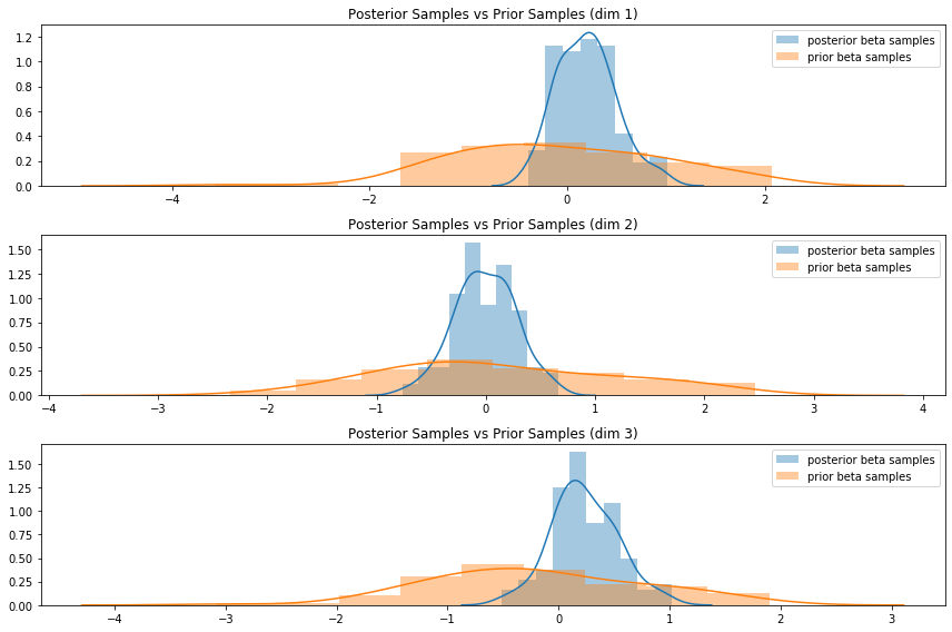
The full details are better explored through the notebook, but my ad-hoc implementation seems to work. First, a quick test to visually confirm that the posterior on an artificially-generated dataset has a lower degree of dispersion compared to the prior:

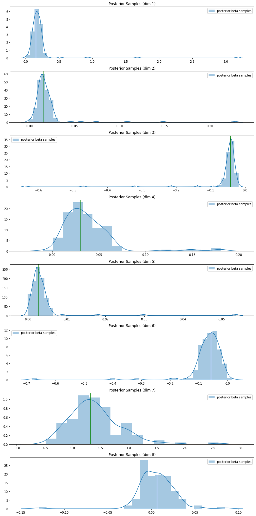
Then, on the Pima Indian diabetes data, I used a normal prior for the weights and ran the above Gibbs sampler to construct a posterior density for the parameters. I plotted the maximum-likelihood estimates (from sklearn’s logistic regression module) for each weight on top of the sampler-constructed posterior for that weight:

Conclusion

Through the above, we can see that the Polya-Gamma distribution permits a flexible bayesian interpretation of the logistic regression model; the original paper by Polson et al actually permits a wider range of discrete binary and count-based regression models to be analyzed through the bayesian framework using the same latent variable data augmentation strategy above. Further investigations are necessary to discover more relevant mathematical properties, but the Polya-Gamma distribution seems to hold a lot of promise for enabling efficient Bayesian inference for a large class of models.

References

• The code corresponding to this post is at https://github.com/paultsw/blogprogs/tree/master/polya_gamma.

• Bayesian inference for logistic models using Polya-Gamma latent variables, Nicholas G. Polson, James G. Scott, Jesse Windle. (ArXiv)

• Bayesian analysis of binary and polychotomous response data, James H. Albert & Siddhartha Chib. (PDF)